urban tree Canopy assessment PROCESS
Davey Resource Group’s Tree Canopy Assessment and Planting Plan for the villages was created using a well-established and statistically rigorous process. First, a land cover extraction was completed using the 2018 National Agriculture Imagery Program (NAIP) photography. A series of random plots were generated and manually inspected to ensure accuracy. As an added level of comparison, Davey Resource Group completed an i-Tree Canopy assessment, which closely reflected the results of the comprehensive land cover extraction. Next, the canopy data from the land cover extraction were analyzed using i-Tree models to generate an estimate of ecosystem benefits provided by the existing tree canopy. Finally, a realistic estimate of potential canopy was created by eliminating areas unsuitable for planting (e.g., impervious surfaces, sports fields). These data were used to develop recommendations to strategically use trees to mitigate stormwater and maximize community benefits.
This study used a variety of data, tools, and analytical methodologies from various sources, including United States Department of Agriculture aerial imagery, census data, remote sensing technology, locally supplied data, scientific studies, and previous canopy analyses. These sources are briefly mentioned or referenced throughout this report.
This study used a variety of data, tools, and analytical methodologies from various sources, including United States Department of Agriculture aerial imagery, census data, remote sensing technology, locally supplied data, scientific studies, and previous canopy analyses. These sources are briefly mentioned or referenced throughout this report.
CLASSIFICATION METHODOLOGY
Davey Resource Group utilized an object-based image analysis (OBIA) semi-automated feature extraction method to process and analyze current high-resolution color infrared (CIR) aerial imagery and remotely-sensed data to identify tree canopy cover and land cover classifications. The use of imagery analysis is cost-effective and provides a highly accurate approach to assessing your community's existing tree canopy coverage. This supports responsible tree management, facilitates community forestry goal-setting, and improves urban resource planning for healthier and more sustainable urban environments
Advanced image analysis methods were used to classify, or separate, the land cover layers from the overall imagery. The semi-automated extraction process was completed using Feature Analyst, an extension of ArcGIS®. Feature Analyst uses an object-oriented approach to cluster together objects with similar spectral (i.e., color) and spatial/contextual (e.g., texture, size, shape, pattern, and spatial association) characteristics. The land cover results of the extraction process was post-processed and clipped to each project boundary prior to the manual editing process in order to create smaller, manageable, and more efficient file sizes. Secondary source data, high-resolution aerial imagery provided by each UTC city, and custom ArcGIS® tools were used to aid in the final manual editing, quality checking, and quality assurance processes (QA/QC). The manual QA/QC process was implemented to identify, define, and correct any classification or omission errors in the final land cover layer.
Advanced image analysis methods were used to classify, or separate, the land cover layers from the overall imagery. The semi-automated extraction process was completed using Feature Analyst, an extension of ArcGIS®. Feature Analyst uses an object-oriented approach to cluster together objects with similar spectral (i.e., color) and spatial/contextual (e.g., texture, size, shape, pattern, and spatial association) characteristics. The land cover results of the extraction process was post-processed and clipped to each project boundary prior to the manual editing process in order to create smaller, manageable, and more efficient file sizes. Secondary source data, high-resolution aerial imagery provided by each UTC city, and custom ArcGIS® tools were used to aid in the final manual editing, quality checking, and quality assurance processes (QA/QC). The manual QA/QC process was implemented to identify, define, and correct any classification or omission errors in the final land cover layer.
CLASSIFICATION WORKFLOW
- Prepare imagery for feature extraction (resampling, rectification, etc.), if needed.
- Gather training set data for all desired land cover classes (canopy, impervious, grass, bare soil, shadows). Water samples are not always needed since hydrologic data are available for most areas. Training data for impervious features were not collected because the city maintained a completed impervious layer.
- Extract canopy layer only; this decreases the amount of shadow removal from large tree canopy shadows. Fill small holes and smooth to remove rigid edges.
- Edit and finalize canopy layer at 1:2,000 scale. A point file is created to digitize-in small individual trees that will be missed during the extraction. These points are buffered to represent the tree canopy. This process is done to speed up editing time and improve accuracy by including smaller individual trees.
- Extract remaining land cover classes using the canopy layer as a mask; this keeps canopy shadows that occur within groups of canopy while decreasing the amount of shadow along edges.
- Edit the impervious layer to reflect actual impervious features, such as roads, buildings, parking lots, etc. to update features.
- Using canopy and actual impervious surfaces as a mask; input the bare soils training data and extract them from the imagery. Quickly edit the layer to remove or add any features. Davey Resource Group tries to delete dry vegetation areas that are associated with lawns, grass/meadows, and agricultural fields.
- Assemble any hydrological datasets, if provided. Add or remove any water features to create the hydrology class. Perform a feature extraction if no water feature datasets exist.
- Use geoprocessing tools to clean, repair, and clip all edited land cover layers to remove any self-intersections or topology errors that sometimes occur during editing.
- Input canopy, impervious, bare soil, and hydrology layers into Davey Resource Group’s Five-Class Land Cover Model to complete the classification. This model generates the pervious (grass/low-lying vegetation) class by taking all other areas not previously classified and combining them.
- Thoroughly inspect final land cover dataset for any classification errors and correct as needed.
- Perform accuracy assessment. Repeat Step 11, if needed.
AUTOMATED FEATURE EXTRACTION FILES
The automated feature extraction (AFE) files allow other users to run the extraction process by replicating the methodology. Since Feature Analyst does not contain all geoprocessing operations that Davey Resource Group utilizes, the AFE only accounts for part of the extraction process. Using Feature Analyst, Davey Resource Group created the training set data, ran the extraction, and then smoothed the features to alleviate the blocky appearance. To complete the actual extraction process, Davey Resource Group uses additional geoprocessing tools within ArcGIS®. From the AFE file results, the following steps are taken to prepare the extracted data for manual editing.
- Davey Resource Group fills all holes in the canopy that are less than 30 square meters. This eliminates small gaps that were created during the extraction process while still allowing for natural canopy gaps.
- Davey Resource Group deletes all features that are less than 9 square meters for canopy (50 square meters for impervious surfaces). This process reduces the amount of small features that could result in incorrect classifications and also helps computer performance.
- The Repair Geometry, Dissolve, and Multipart to Singlepart (in that order) geoprocessing tools are run to complete the extraction process.
- The Multipart to Singlepart shapefile is given to GIS personnel for manual editing to add, remove, or reshape features.
ACCURACY ASSESSMENT PROTOCOL
Determining the accuracy of spatial data is of high importance to Davey Resource Group and our clients. To achieve the best possible result, Davey Resource Group manually edits and conducts thorough QA/QC checks on all tree canopy and land cover layers. A QA/QC process will be completed using ArcGIS® to identify, clean, and correct any misclassification or topology errors in the final land cover dataset. The initial land cover layer extractions will be edited at a 1:2,000 quality control scale in the urban areas and at a 1:2,500 scale for rural areas utilizing the most current high-resolution aerial imagery to aid in the quality control process.
|
To test for accuracy, random plot locations are generated throughout the city area of interest and verified to ensure that the data meet the client standards. Each point will be compared with the most current NAIP high-resolution imagery (reference image) to determine the accuracy of the final land cover layer. Points will be classified as either correct or incorrect and recorded in a classification matrix. Accuracy will be assessed using four metrics: overall accuracy, kappa, quantity disagreement, and allocation disagreement. These metrics are calculated using a custom Excel® spreadsheet.
|
|
LAND COVER ACCURACY
The following describes Davey Resource Group’s accuracy assessment techniques and outlines procedural steps used to conduct the assessment. The tables shown in this section are examples from Ferrysburg's Urban Tree Canopy Assessment. A similar validation process was completed for each community and can be provided if needed.
- Random Point Generation – Using ArcGIS, 750 random assessment points are generated.
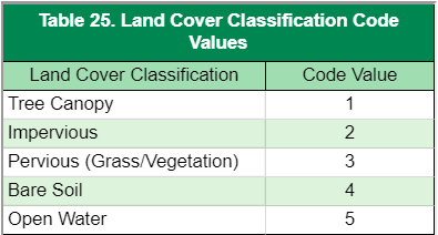
- Point Determination – Each point is carefully assessed by the GIS analyst for likeness with the aerial photography. To record findings, two new fields, CODE and TRUTH, are added to the accuracy assessment point shapefile. CODE is a numeric value (1–5) assigned to each land cover class (Table 25) and TRUTH is the actual land cover class as identified according to the reference image. If CODE and TRUTH are the same, then the point is counted as a correct classification. Likewise, if the CODE and TRUTH are not the same, then the point is classified as incorrect. In most cases, distinguishing if a point is correct or incorrect is straightforward. Points will rarely be misclassified by an egregious classification or editing error. Often incorrect points occur where one feature stops and the other begins
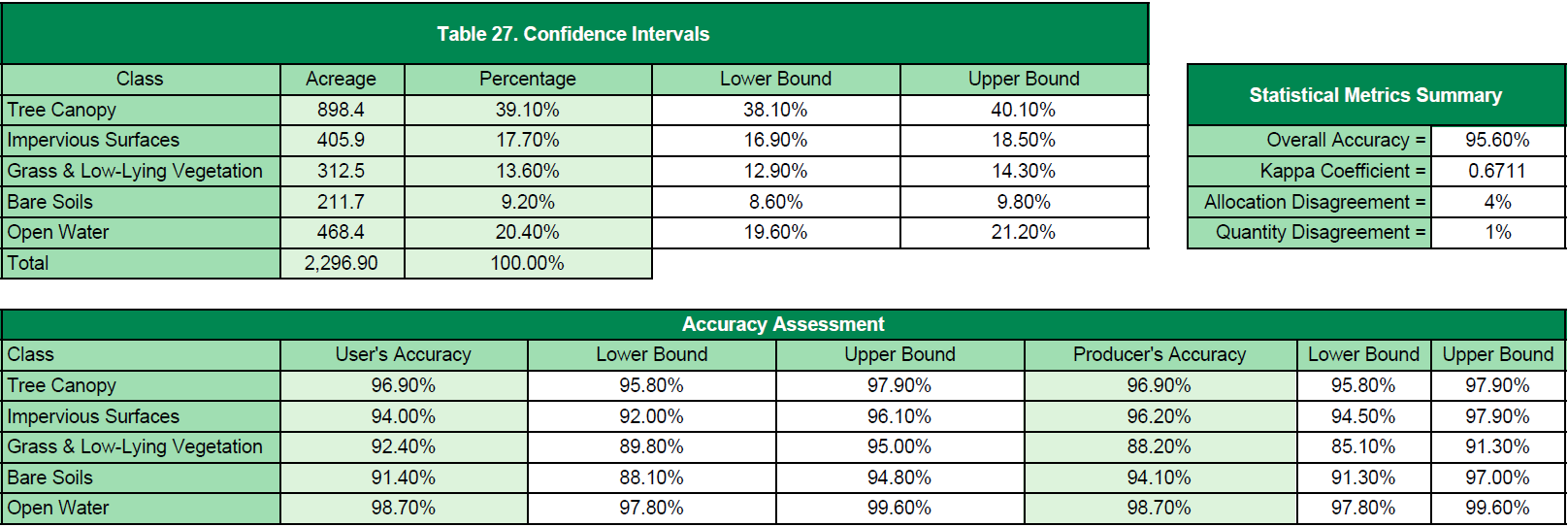
- Classification Matrix – During the accuracy assessment, if a point is considered incorrect, it is given the correct classification in the TRUTH column. Points are first assessed on the NAIP imagery for their correctness using a “blind” assessment—meaning that the analyst does not know the actual classification (the GIS analyst is strictly going off the NAIP imagery to determine cover class). Any incorrect classifications found during the “blind” assessment are scrutinized further using sub-meter imagery provided by the client to determine if the point was incorrectly classified due to the fuzziness of the NAIP imagery or an actual misclassification. After all random points are assessed and recorded; a classification (or confusion) matrix is created. The classification matrix for this project is presented in Table 26. Again, this table is from Ferrysburg's assessment. The other communities have similar tables that can be provided if needed. The table allows for assessment of user’s/producer’s accuracy, overall accuracy, omission/commission errors, kappa statistics, allocation/quantity disagreement, and confidence intervals (Table 27).
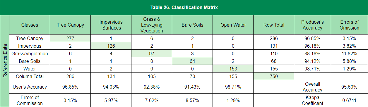
4. Following are descriptions of each statistic as well as the results from some of the accuracy assessment tests.
- Overall Accuracy – Percentage of correctly classified pixels; for example, the sum of the diagonals divided by the total points ((494+71+150+4+5)/750 = 96.53%).
- User’s Accuracy – Probability that a pixel classified on the map actually represents that category on the ground (correct land cover classifications divided by the column total [494/502 = 98.41%]).
- Producer’s Accuracy – Probability of a reference pixel being correctly classified (correct land cover classifications divided by the row total [494/511 = 96.67%]).
- Kappa Coefficient – A statistical metric used to assess the accuracy of classification data. It has been generally accepted as a better determinant of accuracy partly because it accounts for random chance agreement. A value of 0.80 or greater is regarded as “very good” agreement between the land cover classification and reference image.
- Errors of Commission – A pixel reports the presence of a feature (such as trees) that, in reality, is absent (no trees are actually present). This is termed as a false positive. In the matrix below, we can determine that 1.59% of the area classified as canopy is most likely not canopy.
- Errors of Omission – A pixel reports the absence of a feature (such as trees) when, in reality, they are actually there. In the matrix below, we can conclude that 3.33% of all canopy classified is actually present in the land cover data.
- Allocation Disagreement – The amount of difference between the reference image and the classified land cover map that is due to less than optimal match in the spatial allocation (or position) of the classes.
- Quantity Disagreement – The amount of difference between the reference image and the classified land cover map that is due to less than perfect match in the proportions (or area) of the classes.
- Confidence Intervals – A confidence interval is a type of interval estimate of a population parameter and is used to indicate the reliability of an estimate. Confidence intervals consist of a range of values (interval) that act as good estimates of the unknown population parameter based on the observed probability of successes and failures. Since all assessments have innate error, defining a lower and upper bound estimate is essential.
Ecosystem Services MEthodology
Air Quality
The i-Tree Canopy v6.1 Model was used to quantify the value of ecosystem services for air quality. i-Tree Canopy was designed to give users the ability to estimate tree canopy and other land cover types within any selected geography. The model uses the estimated canopy percentage and reports air pollutant removal rates and monetary values for carbon monoxide (CO), nitrogen dioxide (NO2), ozone (O3), sulfur dioxide (SO2), and particulate matter (PM) (Hirabayashi 2014).
Within the i-Tree Canopy application, the U.S. EPA’s BenMAP Model estimates the incidence of adverse health effects and monetary values resulting from changes in air pollutants (Hirabayashi 2014; US EPA 2012). Different pollutant removal values were used for urban and rural areas. In i-Tree Canopy, the air pollutant amount annually removed by trees and the associated monetary value can be calculated with tree cover in areas of interest using BenMAP multipliers for each county in the United States.
To calculate ecosystem services for the study area, canopy percentage metrics from UTC land cover data performed during the assessment were transferred to i-Tree Canopy. Those canopy percentages were matched by placing random points within the i-Tree Canopy application. Benefit values were reported for each of the five listed air pollutants.
Carbon Storage and Sequestration
The i-Tree Canopy v6.1 Model was used to quantify the value of ecosystem services for carbon storage and sequestration. i-Tree Canopy was designed to give users the ability to estimate tree canopy and other land cover types within any selected geography. The model uses the estimated canopy percentage and reports carbon storage and sequestration rates and monetary values. Methods on deriving storage and sequestration can be found in Nowak et al. 2013.
To calculate ecosystem services for the study area, canopy percentage metrics from UTC land cover data performed during the assessment were transferred to i-Tree Canopy. Those canopy percentages were matched by placing random points within the i-Tree Canopy application. Benefit values were reported for carbon storage and sequestration.
Stormwater
The i-Tree Hydro v5.0 Model was used to quantify the value of ecosystem services for stormwater runoff. i-Tree Hydro was designed for users interested in analysis of vegetation and impervious cover effects on urban hydrology. This most recent version (v5.0) allows users to report hydrologic data on the city level rather than just a watershed scale giving users more flexibility. For more information about the model, please consult the i-Tree Hydro v5.0 manual (http://www.itreetools.org).
To calculate ecosystem services for the study area, land cover percentages derived for the project area and all municipalities that were included in the project area were used as inputs into the model. Precipitation data from 2005-2012 was modeled within the i-Tree Hydro to best represent the average conditions over an eight year time period. Model simulations were run under a Base Case as well as an Alternate Case. The Alternative Case set tree canopy equal to 0% and assumed that impervious and vegetation cover would increase based on the removal of tree canopy. Impervious surface was increased 1.7% based on a percentage of the amount of impervious surface under tree canopy and the rest was added to the vegetation cover class. This process was completed to assess the runoff reduction volume associated with tree canopy since i-Tree Hydro does not directly report the volume of runoff reduced by tree canopy. The volume (in cubic meters) was converted to gallons to retrieve the overall volume of runoff avoided by having the current tree canopy.
Through model simulation, it was determined that tree canopy decreases the runoff volume in the project area by 19,194,529 gallons per year using precipitation data from 2005-2012. This equates to approximately 15,586 gallons per acre of tree canopy (19,194,529 gals/15,586 acres).
To place a monetary value on storm water reduction, the cost to treat a gallon of storm/waste water was taken from McPherson et al 1999. This value was $0.089 per gallon. Tree canopy was estimated to contribute roughly $1,708,313 to avoided runoff annually to the project area.
Prioritized planting methodology
|
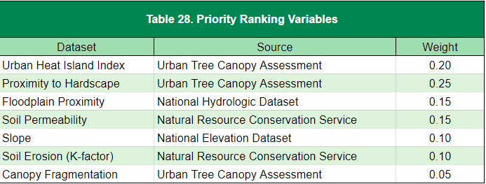
Planting Location The planting location polygons were created by taking all grass/open space and bare ground areas and combining them into one dataset. Non-feasible planting areas such as agricultural fields, recreational fields, major utility corridors, airports, etc. were removed from consideration. The remaining planting space was consolidated into a single feature and, then, exploded back out to multipart features creating separate, distinct polygons for each location. Using zonal statistics, the priority grid raster was used to calculate an average value for each planting location polygon. The averages were binned into five (5) classes with the higher numbers indicating higher priority for planting. These classes ranged from Very Low to Very High. |
|
How Sites Were Prioritized
To identify and prioritize planting potential, Davey Resource Group assessed a number of environmental features, including proximity to hardscape, canopy fragmentation, floodplain proximity, soil permeability, slope, soil erosion factor (K-factor), and urban heat island index. Each factor was assessed using data from various sources and analyzed using separate grid maps. Values between zero and four (with zero having the lowest priority) were assigned to each grid assessed. The grids were overlain and the values were averaged to determine the priority levels at an area on the map. A priority ranging from Very Low to Very High was assigned to areas on the map based on the calculated average of all grid maps.
Once the process of identifying priority was completed, the development of planting strategies was the next task. All potential planting sites were not treated equal as some sites were considered to be more suitable than others. Through prioritization, sites were ranked based on a number of factors pertaining to stormwater reduction and a relative urban heat island index. While available planting sites may ultimately be planted over the next several decades, the trees that are planted in the next several years, should be planned for areas in most need, and where they will provide the most benefits and return on investment.
To identify and prioritize planting potential, Davey Resource Group assessed a number of environmental features, including proximity to hardscape, canopy fragmentation, floodplain proximity, soil permeability, slope, soil erosion factor (K-factor), and urban heat island index. Each factor was assessed using data from various sources and analyzed using separate grid maps. Values between zero and four (with zero having the lowest priority) were assigned to each grid assessed. The grids were overlain and the values were averaged to determine the priority levels at an area on the map. A priority ranging from Very Low to Very High was assigned to areas on the map based on the calculated average of all grid maps.
Once the process of identifying priority was completed, the development of planting strategies was the next task. All potential planting sites were not treated equal as some sites were considered to be more suitable than others. Through prioritization, sites were ranked based on a number of factors pertaining to stormwater reduction and a relative urban heat island index. While available planting sites may ultimately be planted over the next several decades, the trees that are planted in the next several years, should be planned for areas in most need, and where they will provide the most benefits and return on investment.
References
Hirabayashi, S. 2014. i-Tree Canopy Air Pollutant Removal and Monetary Value Model Descriptions. http://www.itreetools.org/canopy/resources/iTree_Canopy_Methodology.pdf [Accessed 11 February 2019]
i-Tree Canopy v6.1. i-Tree Software Suite. [Accessed 11 February 2019] http://www.itreetools.org/canopy
i-Tree Hydro v6.0. i-Tree Software Suite. [Accessed 11 February 2019] http://www.itreetools.org/hydro/index.php
McPherson, E.G.; Simpson, J.R.; Peper, P.J.; Xiao, Q. 1999. Tree Guidelines for San Joaquin Valley Communities. U.S. Department of Agriculture, Forest Service, Pacific Southwest Research Station, Center for Urban Forest Research.
U.S. Environmental Protection Agency (US EPA). 2012. Environmental Benefits Mapping and Analysis Program (BenMAP). http://www.epa.gov/air/benmap [Accessed 11 February 2019]
U.S. Forest Service. 2012. STRATUM Climate Zones. [Accessed 11 February 2019] http://www.fs.fed.us/psw/programs/uesd/uep/stratum.shtml
Hirabayashi, S. 2014. i-Tree Canopy Air Pollutant Removal and Monetary Value Model Descriptions. http://www.itreetools.org/canopy/resources/iTree_Canopy_Methodology.pdf [Accessed 11 February 2019]
i-Tree Canopy v6.1. i-Tree Software Suite. [Accessed 11 February 2019] http://www.itreetools.org/canopy
i-Tree Hydro v6.0. i-Tree Software Suite. [Accessed 11 February 2019] http://www.itreetools.org/hydro/index.php
McPherson, E.G.; Simpson, J.R.; Peper, P.J.; Xiao, Q. 1999. Tree Guidelines for San Joaquin Valley Communities. U.S. Department of Agriculture, Forest Service, Pacific Southwest Research Station, Center for Urban Forest Research.
U.S. Environmental Protection Agency (US EPA). 2012. Environmental Benefits Mapping and Analysis Program (BenMAP). http://www.epa.gov/air/benmap [Accessed 11 February 2019]
U.S. Forest Service. 2012. STRATUM Climate Zones. [Accessed 11 February 2019] http://www.fs.fed.us/psw/programs/uesd/uep/stratum.shtml